Transformer from scratch
Writing a Transformer from scratch is an educational journey into the inner workings of one of the most influential models in the field of Natural Language Processing. Here’s why focusing on this process can be so beneficial:
Deep Understanding: Utilizing pre-trained models or libraries can often lead to a surface-level understanding of the underlying mechanisms. On the other hand, creating a Transformer model from the ground up facilitates a deep, granular comprehension of each part of this complex architecture. You’ll intimately understand the self-attention mechanism, positional encoding, layer normalization, and the importance of masks, among other concepts, as these are all pieces you’ll have to create and interconnect.
Educational Value: Implementing a Transformer from scratch is akin to a hands-on masterclass in advanced deep learning. It’s an effective method of learning that goes beyond theory, encouraging you to apply knowledge and solve problems as they arise. It enables you to grapple with the practical aspects of model development, including debugging, ensuring computational efficiency, and managing resources—a real-life skill set often omitted in theoretical coursework.
Deeper Insights into NLP: Transformers form the backbone of modern NLP, powering applications from translation to text generation. By building a Transformer yourself, you’ll gain insights into why they’re so effective for handling language data and how different components contribute to their exceptional performance. This can be a stepping stone to further explorations and innovations in NLP.
Insight into Generative AI: Transformers have revolutionized not just NLP, but the broader domain of generative AI as well. They lie at the core of cutting-edge models like GPT-3 that can generate human-like text, and have also found applications in areas like music and image generation. By constructing a Transformer from scratch, you’ll gain a foundational understanding of the principles that drive these powerful generative models. This equips you to participate in and contribute to the ongoing advancements in this rapidly evolving field, whether by optimizing existing generative models or pioneering new approaches.
In conclusion, while using pre-built models has its advantages, nothing quite matches the depth of understanding and learning achieved by building a Transformer model from scratch. It’s an endeavor that requires dedication and effort, but the resultant knowledge and skills gained make it a worthwhile investment for any serious learner or practitioner in the field of NLP.
I have decided to embark on this journey of building a Transformer from scratch, inspired by the significant advancements and prolific literature available in the field. There’s a rich body of resources and scholarly articles, tutorials, and code repositories that break down the complexity of the Transformer architecture, serving as invaluable guides and references. I’m particularly grateful to those brave pioneers who ventured into uncharted territory and shared their experiences and insights. Their work has illuminated the path for others and has been instrumental in making these complex concepts more accessible to the broader AI community. Through this endeavor, I hope to deepen my own understanding of Transformer models, while also contributing to the growing body of knowledge on this subject.
Getting Started with Transformers
I am familiar with Pytorch and I will be using it to build the Transformer, but you can use any framework you prefer. As a developer, I find it helpful to have a clear plan of action before starting a project. This helps me stay focused and motivated, and also ensures that I don’t get lost in the details. The famous paper (Attention is all you need) is a must read. I will be using the same notation as the paper as much as possible, so it’s important to understand the terminology and notation used in the paper. I will also be using the same variable names as the paper, so it’s helpful to have the paper open as a reference while going thru is Jupyter Notebook. Here’s the high-level plan I’ve laid out for this project:
I will start by building the core components of the Transformer architecture, which I will combine to create the complete the Transformer model. From a high-level I have decided to build the following components:
Multi-head attention
Transformer Block (which is used in Encoder and Decoder)
Encoder
Decoder block which uses the Transformer Block and Multi-head attention
Decoder
And finally Transformer which uses the Encoder and Decoder
Every component mentioned above will be:
Defined as a
nn.Modulesubclass. This will allow me to leverage the built-in capabilities of PyTorch, including the ability to track and update the model parameters, compute gradients, and more.Have a corresponding unit test to ensure that it’s working as expected. I will also use the unit tests to debug the code and fix any bugs that arise.
Have a
mermaiddiagram to visualize the flow of data. I will use the diagrams to ensure that the dimensions of tensors match at each step, and as a visual aid to understand the model architecture.
Without further ado, let’s begin!
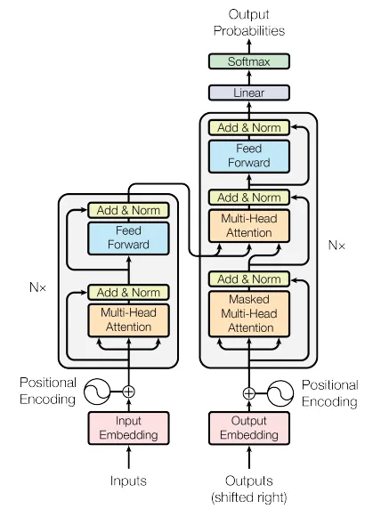
But before we start, how does the data flow in a Transformer?
Assume you have a trained Transformer model that can translate English sentences to French. Here’s how the data flows through the model during prediction:
Source Token Sequence: This is your input sentence in English, tokenized into a sequence of word vectors. The model reads this sequence to understand the context of the input sentence. Assuming N=1 (N is the batch number or the number of sentences in the input), the shape of the tensor is (1, SeqLength), where SeqLength is the length of the sequence or the number of tokens in the English sentence.
Source Mask: This is applied to the source sequence. The purpose of the source mask is to prevent the attention mechanism from focusing on irrelevant parts of the input, such as padding tokens. In a batch of sequences, not all sequences will be of the same length. To make them uniform in length, padding tokens are added to the shorter sequences. These padded positions don’t carry any meaningful information, and it’s important to prevent the self-attention mechanism from considering these positions. A padding mask is used for this purpose. It is typically a tensor with values that are either 0 (for padding positions) or 1 (for actual data positions).
Encoder: The encoder processes the source token sequence and the source mask. Since we are in inference mode, the model isn’t being trained, so the weights remain the same. The encoder’s role is to create a rich representation of the source sentence that captures the semantic information of the input.
Target Token Sequence: At the start of the decoding process, this sequence contains only a start-of-sequence token (in this case for the French language translation). The goal of the model is to generate the rest of the sequence, token by token, which will form our translated sentence in French.
Target Mask: This mask ensures that the prediction for each position can depend only on known outputs at earlier positions, not on future positions, maintaining the auto-regressive property.
Decoder: The decoder processes the output from the encoder, the initial target token sequence, and the target and source masks. It then generates a probability distribution for the next token (the next word in the French translation).The token (word) with the highest probability is selected and added to the target sequence. This updated target sequence is then fed back into the decoder, and the process is repeated. This generation continues until an end-of-sequence token is produced or the sequence reaches a predefined maximum length.
This way, during inference/prediction mode, our English-to-French Transformer model generates a French translation of the input English sentence, one word at a time, based on both the original English sentence and the French words it has generated so far.
graph TB
SRC[Source Token Sequence] --shape=N,SeqLength-->  ENC[Encoder]
SRCM[Source Mask] --> ENC
ENC --shape=N,SeqLength,E--> DEC[Decoder]
TRG[Target Token Sequence] --shape=N,SeqLength-->  DEC
SRCM --> DEC
TRGM[Target Mask] --> DEC
DEC --shape=N,SeqLength,E--> O[Output]
(in case mermaid diagrams are not rendered, here’s the image)
![]()
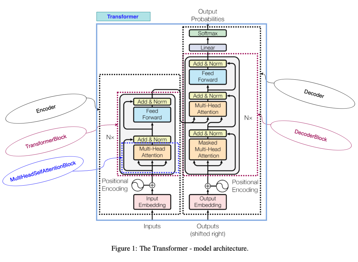
Multti-ead Self Attention Block
You can find implementation here
In machine learning, particularly in models such as Transformers, an attention function is a crucial component that enhances the model’s ability to focus on specific parts of the input data that are relevant for a given task.
Here’s an expanded explanation of the key concepts:
Query, Keys, and Values: These are terms used in the attention mechanism. The ‘query’ is a vector that represents the current item or context we’re focusing on. ‘Keys’ are vectors that represent the different items or contexts available in the input data. ‘Values’ are vectors that represent the actual content or information associated with each key. They query and keys always have the same dimension, but the values can have the same or different dimension.
Compatibility Function: The weights assigned to each value in the weighted sum are determined by a ‘compatibility function’. This is a function that takes the query and a key as inputs, and outputs a score that represents how well the query and key match. This score is then used as the weight for the corresponding value in the weighted sum. In other words, if the query matches well with a certain key (i.e., the compatibility function gives a high score), then the corresponding value gets a high weight, and therefore has a larger influence on the output of the attention function. This is how the attention mechanism allows the model to focus on the most relevant parts of the input data.
Attention Function: This is essentially a mapping procedure. It maps a query (a representation of the current context or focus) and a set of key-value pairs (representations of the possible inputs and their corresponding outputs or ‘values’) to an output.
Weighted Sum of Values: The output of the attention function is calculated as a weighted sum of the values. This means each value vector is multiplied by a certain weight, and then all of these weighted values are added together to produce the output. The idea is to give more ‘attention’ (i.e., higher weight) to the values that are more relevant or useful for the current task.
$$\text{Attention}(Q, K, V) = \text{softmax}\left(\frac{QK^T}{\sqrt{d_k}}\right)V$$
Multi-Head Attention: The multi-head attention mechanism is a variant of the attention mechanism that allows the model to jointly attend to information from different embedding/representation subspaces at different positions. This is beneficial as it allows the model to learn more robust relationships between the query and the key-value pairs. It also helps the model to focus on different positions and subspaces of the input data at different layers of the model.
$$\text{MultiHead}(Q, K, V) = \text{Concat}(\text{head}1, …, \text{head}h)W_O$$ $$\text{where} \quad \text{head}i = \text{Attention}(QW{Qi}, KW{Ki}, VW{Vi})$$
The projections are defined by parameter matrices:
$W_{Qi} \in \mathbb{R}^{E_{\text{model}} \times E_q}$
$W_{Ki} \in \mathbb{R}^{E_{\text{model}} \times E_k}$
$W_{Vi} \in \mathbb{R}^{E_{\text{model}} \times E_v}$
$W_O \in \mathbb{R}^{h E_v \times E_{\text{model}}}$
In our implementation, we use $h=8$ parallel attention layers, also known as heads. For each of these, we set
$E_k = E_q = E_v = E_{\text{model}} / h = 64$.
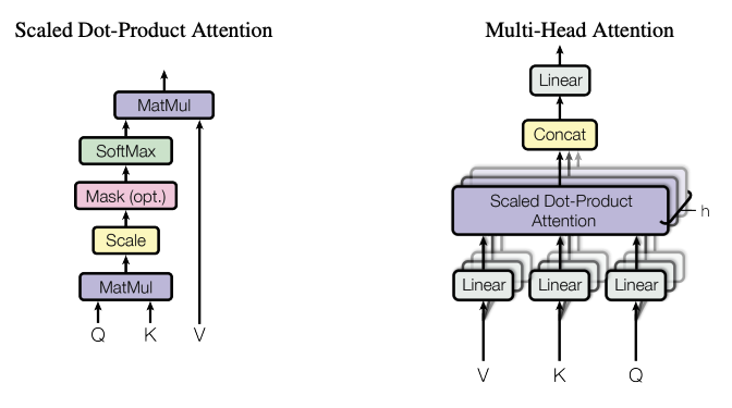
Input
Values(N,Sv,E), Keys(N,Sk,E), Queries(N,Sq,E): they are three tensors “Values”, “Keys”, “Queries” which are linearly transformed to the same embedding size “E”. Keys and Queries have the same shape, while Values can have a different shape (the number of sequences “Sv” can be different from the number of sequences in Keys and Queries “Sk”)
N: Batch Size
Sv, Sk, Sq: Sequence Lengths of Values, Keys, Queries
E: Embedding Size
Mask (Optional)one of two types:
Target Mask: The mask is used to prevent the model from attending to the future tokens. It is a tensor of shape (N, 1, Sq, Sq) where the future tokens are set to 0 and the rest to 1.
Source Mask: The mask is used to prevent the model from attending to the padding tokens. It is a tensor of shape (N, 1,1,Sq/Sk) where the padding tokens are set to 0 and the rest to 1.
graph TB

V[Values] -- shape=N,Sv,E--> B[Linear]
K[Keys] --shape=N,Sk,E--> C[Linear]
Q[Queries] --shape=N,Sq,E--> D[Linear]
B --Values=N,Sv,E--> E[Reshape Values to N,Sv,H,Hd]
C --Keys=N,Sk,E--> F[Reshape Keys to N,Sk,H,Hd]
D --Queries=N,Sq,E--> G[Reshape Queries to N,Sq,H,Hd]
F --Keys=N,Sk,H,Hd,--> H[Scaled Dot Product]
G --Queries=N,Sq,H,Hd--> H
H --Queries=N,Sq,H,Hd--> U[Mask]
U --> I[Softmax]
I --Softmax=N,H,Sq,Sk--> J[Dot Product]
E --Values=N,Sv,H,Hd--> J
J --Dot Product=N,H,Sq,Sk--> L[Reshape to N,Sq,E or concatenate the heads]
L --MatchingValues=N,Sq,E--> M[Linear]
M --MatchingValues=N,Sq,E--> N[Output]
(in case mermaid diagrams are not rendered, here’s the image)
Transformer Block
You can find implementation here
The forward pass in the Transformer Block is as follows:
MultiHeadSelfAttentionBlock (MHA):
Queries (Q),Keys (K),Values (V), and aMask (M)are inputs to the multi-head self-attention block. The shapes of Q, K, and V are (N, Sq, E), (N, Sk, E), and (N, Sv, E), respectively, where N is the batch size, Sq and Sk are sequence lengths of queries and keys and are typically equal, and E is the embedding size. The mask has shape (N, 1, Sq) or (N, 1, 1, Sq), depending on the mask type. This block computes a weighted sum of the ‘Values’ based on the similarity of ‘Keys’ and ‘Queries’, scaled by the mask.LayerNorm + Dropout (LN1): The output from the MHA and the original Queries (residual connection) are added together and then passed through the first Layer Normalization and Dropout operation to stabilize the outputs and prevent overfitting. The output of this stage retains the shape (N, Sq, E).
FeedForwardBlock (FFN): The output of LN1 is passed through a Feed-Forward Neural Network, which consists of two linear transformations with a ReLU activation in between. It’s here where the model can learn more complex representations.
LayerNorm + Dropout (LN2): The output from the FFN and the output of LN1 (again, a residual connection) are added together, then passed through the second Layer Normalization and Dropout operation. This further stabilizes the outputs and helps prevent overfitting.
Output (O): The output of LN2 becomes the final output of this Transformer block. It has the same shape as the input queries (N, Sq, E) and can be used as input to the next Transformer block in the stack (if any), or can be used for further processing (like a linear transformation to obtain prediction scores for downstream tasks).
This high-level description covers one Transformer block, and in practice, several of these blocks are stacked to form the complete Transformer model. This stacking allows the model to learn more complex patterns and relationships in the data.
graph TB
Q[Queries] --shape=N,Sq,E--> MHA
V[Values] -- shape=N,Sv,E--> MHA[MultiHeadSelfAttentionBlock]
K[Keys] --shape=N,Sk,E--> MHA
M[Mask] --shape=N,1,Sq-or-N,1,1,Sq--> MHA
Q --Queries=N,Sq,E--> LN1[LayerNorm + Dropout]
MHA --Queries=N,Sq,E--> LN1
LN1 --Queries=N,Sq,E--> FFN[FeedForwardBlock with forward expansion]
FFN --Queries=N,Sq,E--> LN2[LayerNorm + Dropout]
LN1 --Queries=N,Sq,E--> LN2
LN2 --Queries=N,Sq,E--> O[Output]
(in case mermaid diagrams are not rendered, here’s the image)
![]()
Encoder
You can find implementation here
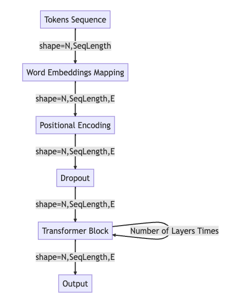
The forward pass in the Encoder is as follows:
Tokens Sequence: The process begins with a sequence of tokens. The shape of this sequence is typically (N, SequenceLength), where N is the batch size and SequenceLength is the length of the sequence for each batch.
Word Embeddings Mapping: The tokens are then passed through an embedding layer that maps each token to a high-dimensional vector. This results in a tensor with shape (N, SequenceLength, E), where E is the dimensionality of the embeddings.
Positional Encoding: Given the lack of inherent sequential information in a Transformer’s architecture, a positional encoding step is applied. This adds information about the position of each token in the sequence to the embedding. The output of this step still maintains the shape (N, SequenceLength, E).
Dropout: To prevent overfitting and improve generalization, a dropout layer is applied. Dropout randomly sets a fraction of input units to 0 at each update during training. The shape remains (N, SequenceLength, E) after this layer as well.
Transformer Block: The processed embeddings are then passed through a Transformer block. The block consists of a self-attention mechanism and a feed-forward neural network, both followed by normalization and dropout. This process could be repeated for a specific number of layers (as Transformers usually consist of multiple such blocks stacked upon each other).
Output: The final output from the Transformer block still maintains the shape (N, SequenceLength, E). This can be used as the input to the next Transformer block in the sequence or to a final linear layer to obtain prediction scores for tasks like sequence classification or translation.
graph TB
X[Tokens Sequence] --shape=N,SeqLength--> W[Word Embeddings Mapping]
W --shape=N,SeqLength,E--> PE[Positional Encoding]
PE --shape=N,SeqLength,E--> DO[Dropout]
DO --shape=N,SeqLength,E--> T[Transformer Block]
T --Number of Layers Times--> T
T --shape=N,SeqLength,E--> O[Output]
(in case mermaid diagrams are not rendered, here’s the image)
Decoder Block
You can find implementation here
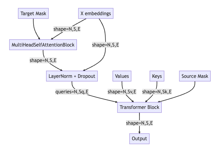
The decoder block uses the same components as the encoder block, such as Multi-head attention, Layer Normalization, and Feed-Forward Neural Network. However, it also has a few additional components, such as the encoder-decoder attention block and the target mask. The forward pass in the Decoder block is as follows:
Target Mask & X embeddings: The decoder block starts by receiving the target mask and the embeddings of the target sequence. The target mask is used to prevent the model from peaking at future positions in the sequence, enforcing the auto-regressive property. The shape of the embeddings (X) is (N, S, E), where N is the batch size, S is the sequence length, and E is the embedding size.
MultiHeadSelfAttentionBlock (MHA): The embeddings and the target mask are passed to a MultiHeadSelfAttentionBlock. This module applies self-attention to the embeddings, taking into account the target mask to avoid peaking at future positions.
LayerNorm + Dropout (LN1): The output of the self-attention block (which still has shape (N, S, E)) is then normalized and subjected to dropout to prevent overfitting. The input embeddings X are also added back to the output of the self-attention block, in a “residual connection” that helps to mitigate the vanishing gradients problem in deep networks.
Transformer Block (TR): The output from the previous layer serves as the queries to the Transformer Block. It also receives the keys (K) and values (V), which typically are the outputs of the encoder. Additionally, the source mask is applied, which prevents the decoder from attending to specific positions in the source sequence (for example, padding positions).
Output (O): Finally, the output from the Transformer Block is forwarded. This is typically passed through a linear layer followed by a softmax to produce probability scores for each token in the target vocabulary. The shape of this output is still (N, S, E), maintaining the batch size, sequence length, and embedding size dimensions.
graph TB
T[Target Mask] --> MHA[MultiHeadSelfAttentionBlock]
X[X embeddings] --shape=N,S,E--> MHA

MHA --shape=N,S,E--> LN1[LayerNorm + Dropout]
X --shape=N,S,E--> LN1
LN1 --queries=N,Sq,E--> TR[Transformer Block]
V[Values] --shape=N,Sv,E--> TR
K[Keys] --shape=N,Sk,E--> TR
S[Source Mask] --> TR
TR --shape=N,S,E--> O[Output]
(in case mermaid diagrams are not rendered, here’s the image)
Decoder
You can find implementation here
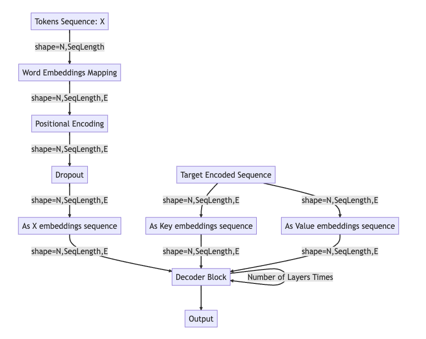
In decoder the forward pass is as follows:
Tokens Sequence: The target sequence, denoted as X, is the input to the decoder. Its shape is (N, SeqLength), where N is the batch size and SeqLength is the sequence length.
Word Embeddings Mapping: The input sequence X is passed through an embedding layer that transforms each token into a dense vector of size E. The resulting shape is (N, SeqLength, E), where E is the embedding size.
Positional Encoding: Positional encoding is added to these embeddings to encode the order of the tokens in the sequence, since this information is not inherently captured in the self-attention mechanism.
Dropout: A dropout layer is applied to prevent overfitting and to add some noise to the data.
As X embeddings sequence (identity): The output from the dropout layer serves as the initial sequence of embeddings X for the decoder block.
Target Encoded Sequence: The encoded sequence (Y), typically the output of the encoder, is processed to be used as the keys and values for the attention mechanism in the decoder. They are of shape (N, SeqLength, E).
As Key/Value embeddings sequence (identity): The encoded sequence is used directly as keys (ASK) and values (ASV), with the same shape of (N, SeqLength, E).
Decoder Block: The decoder block receives the input embeddings sequence X, the key embeddings ASK, and the value embeddings ASV. The decoder block applies masked self-attention on X and then applies another attention mechanism using X as queries, ASK as keys and ASV as values.The Decoder Block’s output is then passed through the same series of layers multiple times (the exact number is a parameter of the model), with each pass allowing the decoder to refine its understanding of the input sequence in the context of the output it is generating.
Output: The final output of the Decoder Block, which retains the shape of (N, SeqLength, E), can be used to predict the next token in the target sequence by passing it through a linear layer and then a softmax to generate probability scores for each token in the target vocabulary.
graph TB
X[Tokens Sequence: X] --shape=N,SeqLength-->  WE[Word Embeddings Mapping]
WE --shape=N,SeqLength,E--> PE[Positional Encoding]
PE --shape=N,SeqLength,E--> DO[Dropout]
DO --shape=N,SeqLength,E--> ASX[As X embeddings sequence]
ASX --shape=N,SeqLength,E-->T[Decoder Block]
T --Number of Layers Times--> T
Y[Target Encoded Sequence] --shape=N,SeqLength,E --> ASV[As Value embeddings sequence]
Y --shape=N,SeqLength,E--> ASK[As Key embeddings sequence]
ASK --shape=N,SeqLength,E-->T[Decoder Block]
ASV --shape=N,SeqLength,E-->T[Decoder Block]
T --> O[Output]
(in case mermaid diagrams are not rendered, here’s the image)
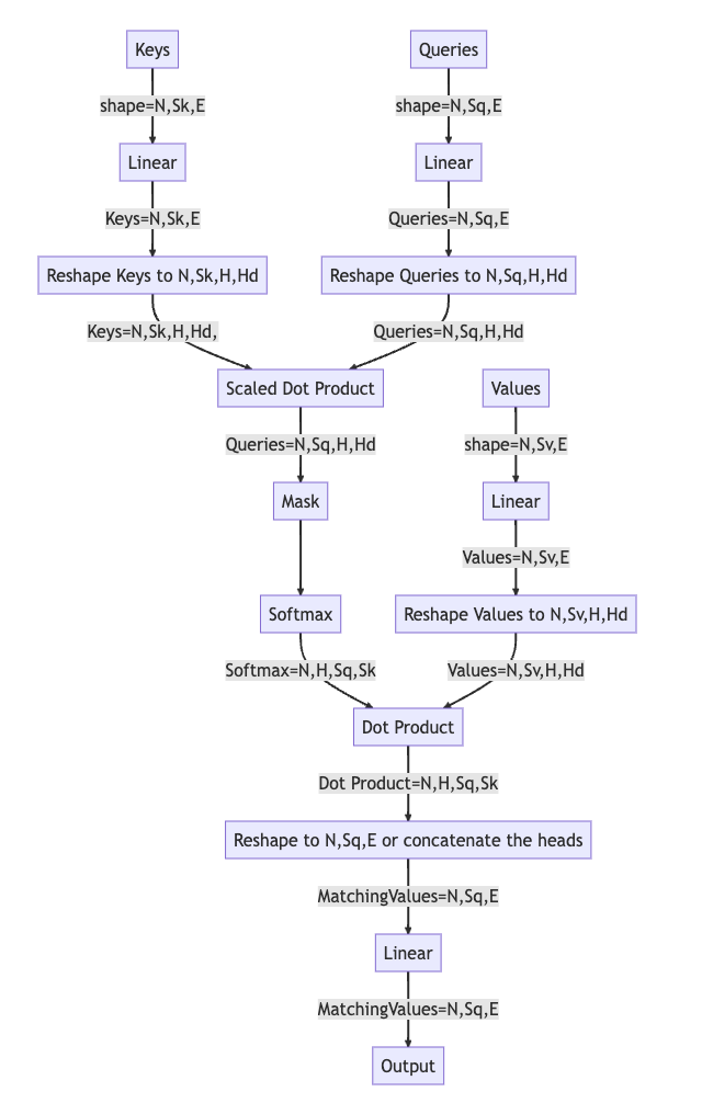
All together now “Transformer”
You can find implementation here
graph TB
SRC[Source Token Sequence] --shape=N,SeqLength-->  ENC[Encoder]
SRCM[Source Mask] --> ENC
ENC --shape=N,SeqLength,E--> DEC[Decoder]
TRG[Target Token Sequence] --shape=N,SeqLength-->  DEC
SRCM --> DEC
TRGM[Target Mask] --> DEC
DEC --shape=N,SeqLength,E--> O[Output]
(in case mermaid diagrams are not rendered, here’s the image)
![]()